|
|
|
| This document is available in: English Deutsch Francais Turkce |
![[Photo of the author]](../../common/images/John-Perr.gif)
by John Perr <johnperr(at)linuxfocus.org> About the author: Linux user since 1994; he is one of the French editors of LinuxFocus. Mechanical Engineer, MSc Sound and Vibration Studies Translated to English by: John Perr <johnperr(at)linuxfocus.org> Content:
|
Basic acoustics and Signal Processing![[Illustration]](../../common/images/article271/illustration271.png)
Abstract:
This is Basic acoustics and Signal Processing for musicians
and computer scientists. |
This article intends to be educational. It hopes to provide the
reader with a basic knowledge of sound and sound processing. Of
course music is one of our concerns but all in all, it is just some
noise among other less pleasant sounds.
First the physical concepts of sound are presented together with
the way the human ear interprets them. Next, signals will be looked
at, i.e. what sound becomes when it is recorded especially with
modern digital devices like samplers or computers.
Last, up to date compressions techniques like mp3 or Ogg vorbis
will be presented.
The topics discussed in this paper should be understandable by a
large audience. The author tried hard to use "normal terminology"
and particularly terminology known to musicians. A few mathematical
formulas pop up here and there within images, but do not matter
here (phew! what a relief...).
Physically speaking, sound is the mechanical vibration of any
gaseous, liquid or solid medium. The elastic property of the
medium allows sound to propagate from the source as waves, exactly
like circles made by a stone dropped in a lake.
Every time an object vibrates, a small proportion of its energy is
lost in the surroundings as sound. Let us say it right now, sound
does not propagate in a vacuum.
Figure 1a shows how a stylus connected to a vibrating source, like
a speaker for example, converts to a wave when a band of paper
moves under it.
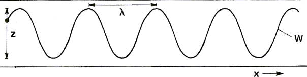
| z: Vibrating stylus of amplitude
±A0 λ: wavelength x: band speed at speed c w: Resulting wave Figure 1a: Vibrating stylus on a moving paper band |
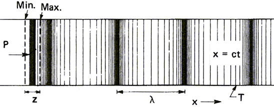
As far as air is concerned, sound propagates as a pressure
variation. A loudspeaker transmits pressure variations to the air
around it. The compression (weak) propagates through the air.
Please note that only the pressure front moves, not the air. For
the circles in water mentioned earlier, waves do move whereas
water stays in the same place. A floating object only moves up and
down. This is why there is no "wind" in front of the loudspeaker.
Sound waves propagate at about 344 meters per second, in air at
20°C, but air particles only move a few microns back and
forth.
We know now, from the above drawings, that sound waves have a
sine shape. Distance between two crests is called wavelength and
the number of crests an observer sees in one second is called
frequency. This term used in physics is nothing but the pitch of a
sound for a musician. Low frequencies yield bass tones whereas high
frequencies yield high pitched tones.
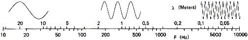
Figure 2 gives values for both frequency and wavelength of sound
waves propagating through the air:
Another characteristic of sound is its amplitude. Sound can be soft or loud. Through the air it corresponds to small or large variation in pressure depending on the power used to compress air. Acousticians use decibels to rate the strength of sound. Decibel is a rather intricate unit as shown on drawings 3a and 3b. It has been chosen because figures are easy to handle and because this logarithmic formula corresponds to the behavior of the human ear as we shall see in the next chapter. Undoubtedly you are doing math without knowing it:
| Figure 3a: Noise level and pressure | Figure 3b: Noise level and power |
Up to now, we only need to know that dB are related to the power
of sound. 0 dB corresponds to the lower threshold of human
hearing and not to the absence of noise. Decibels are a
measure of noise relative to human capabilities. Changing the
reference (Po or Wo) above will change the dB value accordingly.
This is why the dB you can read on the knob of your Hi-Fi amplifier
are not acoustic levels but the amplifier electrical output power.
This is a totally different measure, 0 dB being often the maximum
output power of your amplifier. As far as acoustics is concerned,
the sound level in dB is much greater, otherwise you would not have
bought that particular amplifier, but it also depends on the
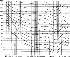
efficiency of you loud speakers... Figure 4 helps you locate a few usual
sound sources both in amplitude and frequency. The curves
represents levels of equal loudness as felt by the human ear; we shall detail
this later:
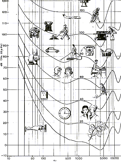
The array below shows levels in decibels and watts of a few usual sound sources. Please note how the use of decibels eases notation:
| Power (Watt) | Level dB | Example | Power (W) |
|---|---|---|---|
| 100 000 000 | 200 | Saturn V Rocket 4 jet air liner |
50 000 000 50 000 |
| 1 000 000 | 180 | ||
| 10 000 | 160 | ||
| 100 | 140 | Large orchestra | 10 |
| 1 | 120 | Chipping hammer | 1 |
| 0.01 | 100 | Shouted speech | 0.001 |
| 0.000 1 | 80 | ||
| 0.000 001 | 60 | Conversational speech | 20x10-6 |
| 0.000 000 01 | 40 | ||
| 0.000 000 000 1 | 20 | Whisper | 10-9 |
| 0.000 000 000 001 | 0 | ||
| Sound power output of some typical sound sources | |||
Sound amplitude can be measured in different ways. This also applies to other wave signals as Figure 5 demonstrate it:
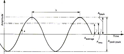
| Symbol | Name | Definition |
|---|---|---|
| Aaverage | Average Amplitude | Arithmetic average of positive signal |
| ARMS | Root mean square | Amplitude proportional to energy content |
| Apeak | Peak Amplitude | Maximal positive amplitude |
| Apeak-peak | Amplitude peak to peak | Maximal positive to negative amplitude |
The average amplitude is only a theoretical measure and technically not used. On the other hand, the root mean square value is universally adopted to measure equivalent signals and especially sine waves. For instance, the equivalent current available on one of your home plugs is rated 220 volts sinusoidal varying at a constant frequency of 50 Hz. Here the 220 volts are RMS volts so that the voltage is really oscillating between -311 volts and +311 volts. Using the other definitions, this signal is 311 volts peak or 622 Volts peak to peak. The same definitions apply for the output of power amplifiers, fed to speakers. An amplifier able to yield 10 watts RMS will have a peak value of 14 watts and a peak to peak value of 28 watts. These peak to peak measurements of sine waves are called musical watts by audio-video retailers because the figures are good selling arguments.
As it does with music, time plays a fundamental role with
acoustics. A very close relationship binds time to space because
sound is a wave that propagates into space over time.
Taking this into account, three classes of acoustic signals are
defined:
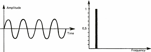
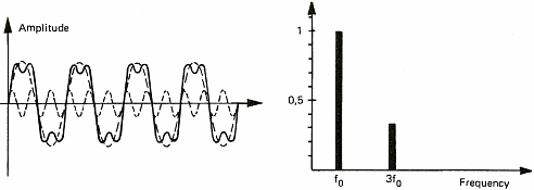
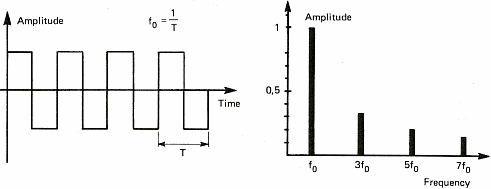
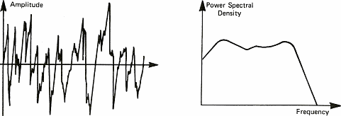
The diagrams of figure 6 show some sound signals. We take advantage of these diagrams to introduce the notion of spectrum. The spectrum of a signal shows the different "notes" or pure sounds that make a complex sound. If we take a stable periodic signal like a siren or a whistle, the spectrum is stable over time and only shows one value (one line on figure 6a). This is because it is possible to consider each sound as the combination of pure sounds which are sine waves. We shall see later on that this decomposition of periodic signals into sine waves has been demonstrated by a French mathematician named Fourier in the 19th century. This will also allow us to talk about chords as far as music is concerned. Meanwhile, I shall stick to sine waves because it is a lot easier to draw than solos from Jimmy Hendrix.
In order to be able to process sound with a computer, we have to acquire it. This operation will allow us to transform the variation in pressure of the air into a series of numbers that computers understand. To do so, one uses a microphone which converts pressure variations into electrical signals and a sampler which convert the electric signal into numbers. A sampler is a general term and ADC (Analog to Digital Converter) is often used by electricians. This task is often devoted to the sound card of personal computers. The speed at which the sound card can record points (numbers) is called the sampling frequency. Figure 7 below shows the influence of the sampling frequency on a signal and its spectrum calculated by mean of the Fourier transform. Formula are here for the math addicts:
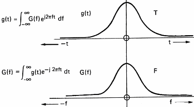
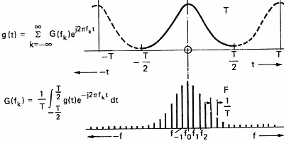
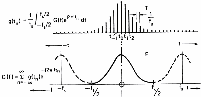
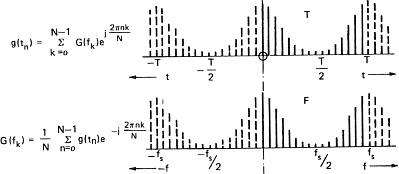
This demonstrates (please believe me) that the transformation of
a continuous wave into a series of discrete points makes the
spectrum periodic. If the signal is also periodic, then the
spectrum is also discrete (a series of points) and we only need to
compute it at a finite number of frequencies. This is a good news
because our computer can only compute numbers and not waves.
So we are now faced with the case of fig. 7d where a sound signal
and its spectrum are both known as a series of points which where the
fluctuate over time and in the frequency domain between 0 Hz and
half the sampling frequency.
All these figures lining up have finally lost some part of the
original sound signal. The computer only knows the sound at some
precise moments. In order to be sure that it will be played
properly and without any ambiguity, we have to be careful while
sampling it. The first thing to do is to be sure that no frequency
(pure sounds) greater than half the sampling frequency is present
in the sampled signal. If not, they will be interpreted as lower
frequencies and it will sound awful. This is shown in figure 8:
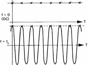
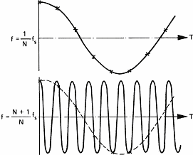
This particular behavior of sampled signals is best known as the Shannon theorem. Shannon is the mathematician who has demonstrated this phenomenon. A similar effect can be observed on the cart wheels in films, e.g westerns. They often appear to run backward because of the stroboscopic effect of films. For daily use of sound acquisition, this means that you need to eliminate all frequencies above half the sampling frequency. Not doing so will mangle the original sound with spurious sounds. Take for instance the sampling frequency of compact discs (44.1 KHz); sounds above 22 KHz must be absent (tell your bats to keep quite because they chat with ultra sounds).
In order to get rid of the unwanted frequencies, filters are used. Filter is a widely used term that applies to any device able to keep or transform partial sound. For example, low pass filters are used to suppress high frequencies which are not audible but annoying for sampling (the gossiping of the bats). Without going into details, the following diagram shows the characteristics of a filter:
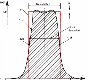
A filter is a device that changes the signal both the time and
spectrum of the sound wave. A 100 Hz square wave low pass filtered
at 200 Hz will become a sine wave because the upper part of its
spectrum is removed (see figure 6c). Similarly, a note at 1000 Hz
played by a piano (C 6) will sound like a whistle if it is filtered
at 1200 or 1500 Hz. The lower frequency of the signal is called
fundamental frequency. The others are multiples and are called
harmonic frequencies.
In the time domain, a filter introduces modifications of the wave
called distortions. This is mainly because of the delay taken by
each harmonic relatively to the others.
In order to show the influence of a filter on a signal, let us consider a simple square pulse (figure 10a),the amplitude of its spectrum (figure 10b) and the phase of its spectrum (figure 10c). This square pulse acts as a filter allowing sound to go through between t=0 and T seconds. The spectrum of the pulse represents the frequency response of the filter. We see that the higher the frequency of the signal, the bigger is the delay between the frequency components and the lower is their amplitude.
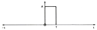
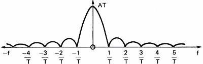
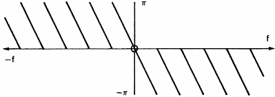
Figure 11 represents the influence of the rectangular filter on a simple signal like a sine wave.
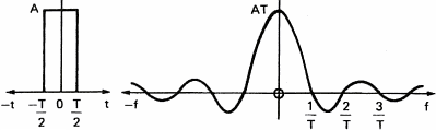
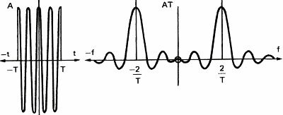
Cutting sound abruptly at time T introduces new frequencies in the spectrum of the sine wave. If the filtered signal is more complex, like the square wave of figure 6c, the frequency components will lag giving a distorted signal on the output of the filter.
For a better understanding of acoustics and sound, let us focus
on the part we use to receive sound: the ear.
Figure 12 shows a cross section of the ear. Sound is collected in
the pinna and channeled through the auditory canal toward the ear
drum which acts more or less like a microphone. The vibrations of
the ear drum are amplified by three small bones acting like levers
and named the hammer, the anvil and the stirrup.
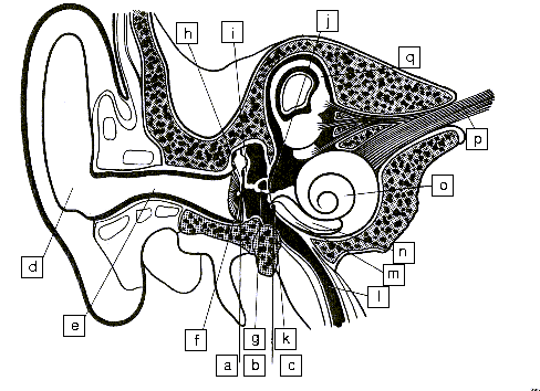 |
a) Outer ear b) Middle ear c) Inner ear d) Pinna e) Ear Canal f) Ear Drum g) Stapes h) Malleus i) Incus j) Oval Window k) Round Window l) Eustachian Tube m) Scala Tympani n) Scala vestibuli o) Cochlea p) Nerve Fiber q) Semicircular canal |
|
| Figure 12: The main parts of the ear | ||
The movements of the stirrup are transmitted via the oval window to the cochlea. The cochlea contains two chambers separated by the basilar membrane which is covered with sensitive hair cells linked to the auditory nerve (As shown on figure 13 and 14 below). The basilar membrane acts as spatial filter because the various parts of the cochlea are sensitive to the various frequencies thus allowing the brain to differentiate the pitch of notes.
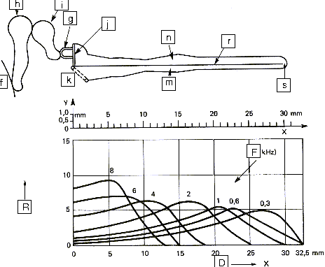 |
f) Ear Drum g) Stirrup h) Hammer i) Anvil j) Oval Window k) Round Window m) Scala Tympani n) Scala vestibuli r) Basilar Membrane s) Helicotrema R) Relative response F) Frequency response D) Distance along membrane |
|
| Figure 13: Longitudinal section of the cochlea | ||
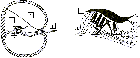 |
m) Scala Tympani n) Scala vestibuli p) Auditive Nerve r) Basilar Membrane t) Scala media u) Hair cell |
|
| Figure 14: Section across the cochlea | ||
The brain plays a very important role because it does all the
analysis work in order to recognize sounds, according to
pitch of course, but also according to duration. The brain
also performs the correlation between both ears in order to locate
sound in space. It allows us to recognize a particular instrument
or person and to locate them in space. It seems that most of the
work done by the brain is learned.
Figure 15 shows how we hear sounds according to frequencies.
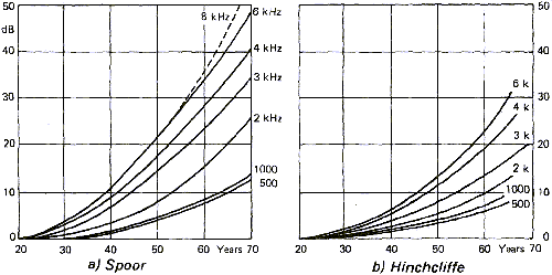
The curves above have been drawn for an average population and are a statistical result for people aged between 18 and 25 and for pure tones. The differences between individuals are explained by many factors among which:
Figure 16 shows the influence of age on hearing loss for different frequencies. According to the sources the results are different. This is explained easily by the large variations that can be observed in a population and because these studies cannot easily take only age into account. It is not rare to find aged musicians with young ears as well as there are young people with important hearing loss due to long exposure to strong noises like those found in concerts or night clubs.
Noise induced hearing loss depends both on the duration of
exposure and on the noise intensity. Note that all sounds are
considered here as "noise" and not only the unpleasant ones. Thus,
listening to loud music with headphones has the same effect on the
auditive cells as listening to planes taking off on the end of
the runway.
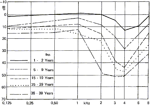
Figure 17 shows the effect of exposure to noise on hearing. Notice
that the effects are not the same as those induced by age where
the ear loses sensitivity at high frequencies. On the other hand,
noise induced hearing loss makes the ear less sensitive around 3-4
Khz. At those frequencies, the ear is the most sensitive. This kind
of hearing loss is usually seen among firearms users.
If you take a look at the chapter about decibels and their
calculation, you will notice that about ten decibels corresponds to a very
large acoustic pressure change. Having a linear decibel scale is
equivalent to an exponential pressure scale. This is because the
ear and the brain are able to handle very large variation of both
amplitude and frequency. The highest frequency sound the healthy
human can ear is 1000 times the frequency the lowest, and the
loudest can have a sound pressure one billion times that of the
quietest that can be heard (an intensity ratio of 1012
to 1).
Doubling pressure only represents 3 dB. This can be heard but an
increase of 9 dB of the sound intensity is needed for the human
being to have a subjective feeling of double volume. This is an
acoustic pressure 8 times stronger!
In the frequency domain, changing octave is equivalent to doubling
the sound frequency. Here too, we hear linearly the exponential
increase of a physical phenomenon. Do not rush to your calculator
yet, calculating the pitches of notes will be done later on.
Recording sound using an analog device like a tape recorder or a vinyl disc is still a common operation even if it tends to be overcome by digital systems. In both cases, transforming a sound wave into magnetic oscillations or digital data, introduces limits inherent to the recording device. We quickly talked earlier about the effects of sampling on the spectrum of sound. Other effects can be expected when recording sound:
"Dynamic" is the term used for a recording device in order to
express the difference between the minimum and maximum amplitude
the device can record. It generally starts with the microphone,
converting sound into an electrical signal, up to the recording
medium, disc, tape or computer...
Remember that decibels do express a ratio. As far as dynamic range
is concerned, the value given is relative to the minimum of the
scale which is 0 dB. Here are a few examples:
A symphonic orchestra can play sounds ranging up to 110 dB. This is why disc editors use dynamic compression systems so that louder sounds are not clipped and quieter ones not lost into noise.
In addition to being less capable than the human ear, recording devices also have the drawback of generating their own noise. It can be the rubbing of the diamond on the vinyl disc or the snoring of the amplifier. This kind of noise is usually very low but do not allow for quietest sounds to be recorded. It is best heard most of the time with good quality headphones and sounds like a waterfall because it has a very wide spectrum including many frequencies.
We saw earlier that filters have an important effect on the
phase of a spectrum because they shift signals according to their
frequency. This type of signal distortion is called harmonic
distortion because it affects the harmonic frequencies of the
signal.
Every single device recording a signal behaves like a filter and
thus induces signal distortions. Of course, the same happens
when you play any recorded sound again. Additional distortion and
noise will be added.
More and more, compression algorithms like mp3 or Ogg Vorbis are
used to gain precious disk space on our recording media.
These algorithms are said to be destructive because they do
eliminate part of the signal in order to minimize space.
Compression programs use a computer model of the human ear in order
to eliminate the inaudible information. For instance, if two
frequency components are close to each other, the quietest can be
safely taken off because it will be masked by the louder one. This
is why tests and advice can be found on the Internet in order to
best use this software, i.e. keep the best part of the signal.
According to those read by the author, most mp3 compressions do
low pass filter sounds at 16 KHz and do not allow for bit rates
higher than 128 KiloBits/seconds. These figures are most of the
time unable to maintain sound at CD quality.
On the other hand, compression software like gzip, bzip2, lha or
zip do not alter data but have lower compression ratios. Moreover,
it is necessary to uncompress the whole file before listening to
it, which is not what is needed for a walkman or any other sound
playing device.
In order to settle things, here is a comparison of terms used by music and science. Most of the time, these comparisons have limits because the terms used by music lovers describe human hearing and not physical phenomenons.
A note is defined, amongst others, by its pitch and this pitch can be assumed to be the fundamental frequency of the note. Knowing this, the frequencies of notes can be calculated with the following formula:
If we use REF for A at 440 Hz from octave 4 as base, we can compute the others for tones ranging from 1 to 12 from C to B:
| Note | Octave | |||||||
|---|---|---|---|---|---|---|---|---|
| 1 | 2 | 3 | 4 | 5 | 6 | 7 | 8 | |
| C | 32,70 | 65,41 | 130,8 | 261,6 | 523,3 | 1047 | 2093 | 4186 |
| C # | 34,65 | 69,30 | 138,6 | 277,2 | 554,4 | 1109 | 2217 | 4435 |
| D | 36,71 | 73,42 | 146,8 | 293,7 | 587,3 | 1175 | 2349 | 4699 |
| E b | 38,89 | 77,78 | 155,6 | 311,1 | 622,3 | 1245 | 2489 | 4978 |
| E | 41,20 | 82,41 | 164,8 | 329,6 | 659,3 | 1319 | 2637 | 5274 |
| F | 43,65 | 87,31 | 174,6 | 349,2 | 698,5 | 1397 | 2794 | 5588 |
| F # | 46,25 | 92,50 | 185,0 | 370,0 | 740,0 | 1480 | 2960 | 5920 |
| G | 49,00 | 98,00 | 196,0 | 392,0 | 784,0 | 1568 | 3136 | 6272 |
| A b | 51,91 | 103,8 | 207,6 | 415,3 | 830,6 | 1661 | 3322 | 6645 |
| A | 55,00 | 110,0 | 220,0 | 440,0 | 880,0 | 1760 | 3520 | 7040 |
| B b | 58,27 | 116,5 | 233,1 | 466,2 | 932,3 | 1865 | 3729 | 7459 |
| B | 61,74 | 123,5 | 246,9 | 493,9 | 987,8 | 1976 | 3951 | 7902 |
The true music lovers will notice that we do not make any
distinction between diatonic or chromatic half tones. With minimal
changes, the same calculations can be done using commas as a
subdivision instead of half tones...
Assuming notes are frequencies is far from being enough to
distinguish a note played by one instrument from another one.. One
also needs to take into account how the note is played (pizzicato or
legato), from which instrument it comes, not counting all
possible effects like glissando, vibrato, etc... For this purpose,
notes can be studied using their sonogram which is their spectrum
across time. A sonogram allows all the harmonic frequencies to be
viewed along time.
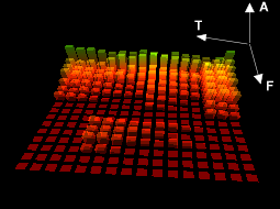
| Figure 18: A sonogram | ||
| T: Time | A: Amplitude | F: Frequency |
Nowadays, electronic sound recording and playing uses totally
artificial devices like synthesizers for creating sounds out of
nothing or samplers to store sound and play it at different pitches
with various effects. It is then possible to play a cello concerto
replacing the instruments with sampled creaking of chairs. Every
body can do it, no need to be able to play any instrument.
The characteristics of a single note are given in the diagram
below:
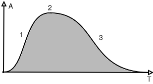
| Figure 19: Characteristics of a note: envelop | |
| 1: Attack | A: Positive Amplitude |
| 2: Sustain | T: Time |
| 3: Decay | |
The curve shows the evolution of the global loudness of sound
along time. This type of curve is called an envelop because it does
envelop the signal (grey part of the drawing). The rising part is
called the attack and can differ tremendously according to the type
of instrument. The second part is called sustain and is the body of
the note and is often the longest part except for percussion
instruments. The third part can also change shape and length
according to the instrument.
Moreover, instruments allow musicians to influence each of the three
parts. Hitting differently the keys of a piano will change the
attack of the note whereas the pedals will change the decay. Each of
the three parts can have its individual spectrum (color) which make
the sound diversity infinite. Harmonic frequencies do not change at
the same rate. Bass frequencies tend to last longer so that the
color of the sound is not the same at the beginning and at the end
of the note.
According to its definition, the frequency range of a device can be associated to the range of an instrument. In both cases the terms describe a range of frequencies or pitches an instrument can play. However, the highest pitch an instrument can play is equivalent to the fundamental frequency given in the array above. In other words, recording a given instrument requires a device having a frequency range much higher to the highest note the instrument can play if the color of the notes are to be recorded. A short frequency range will low pass filter all the upper harmonics of the higher pitch notes and this will change sonority. In practice, a device with the frequency range of the human ear, i.e. 20hz to 20Khz, is needed. Often it is necessary to go higher than 20 Khz, because devices introduce distortion well before the cut off frequency.
Analysing the frequency array of notes above, musicians will
find similarities between harmonic frequencies and notes making a
chord.
Harmonic frequencies are multiples of the fundamental frequency. So
for a C 1 at 32,7 Hz The harmonic frequencies are:
| Harmonic | 1 | 2 | 3 | 4 | 5 | 6 | 7 | 8 |
|---|---|---|---|---|---|---|---|---|
| Frequency | 32,7 | 65,4 | 98,1 | 130,8 | 163.5 | 196,2 | 228,9 | 261,6 |
| Note | C | C | G | C | E | G | B b | C |
Here we see why a chord is known as perfect (C-E-G-C) or seventh (C-E-G-Bb): The frequencies of the notes within the chord are aligned with the harmonic frequencies of the base note (C). This is where the magic is.
Without much going into the details, we have looked at the physical, human and technical aspects of sound and acoustics. This being said, your ear is will always be the best choice criterion. Figures given by mathematics or sophisticated measuring devices can help you understand why one particular record sounds weird but they will never tell you if the Beatles made better music than the Rolling Stones in the sixties.
Brüel & Kjaer: Danish company making measurement instruments for acoustics and vibrations. This company has published for a long time (fifty years or so) free books where most of the drawings for this article come from. These books are available on line in PDF format under the following http://www.bksv.com/bksv/2148.htm link.
|
|
Webpages maintained by the LinuxFocus Editor team
© John Perr, FDL LinuxFocus.org |
Translation information:
|
2003-02-28, generated by lfparser version 2.35